Rotational Kinematics | Angular Position, Velocity, and Acceleration for Non-uniform Circular Motion

Motivation: Rotational Kinematics involves describing the motion of an object moving around in a circle of constant radius. The motion could be described by a set of Cartesian (x and y) coordinates - the motion is inherently in two dimensions - but using the angle to describe position instead simplifies the analysis and still preserves the ability to determine the instantaneous features of the motion. An example is an object that moves from a position $\theta_i$ to a position $\theta_f$, as shown in the diagram below.

Image

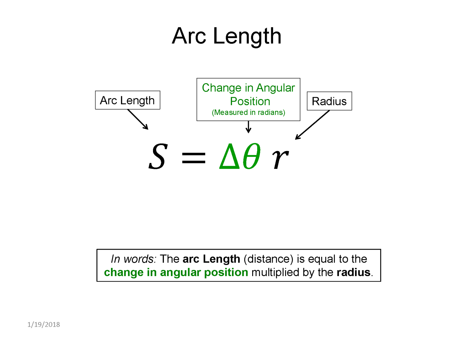
Here you see the change in position can be described by the change in the angle, $\Delta \theta$. If the angles are measured in Radians, which is convention, then the actual distance traveled, called the arc length, is equal to the radius times the change in angle, $s=\Delta \theta r$. This point is made so that you can see that by working with the angular variable $\theta$, measured in Radians, we can still go back to the linear counterpart distance, measured in meters. For now I think it is best to concentrate only on the angular variables and in the end I'll show how all of them can be used to determine their linear counterparts.

Rotational Kinematic Variables:

Angular Position: $\theta$, Change in Angular Position: $\Delta \theta$, Angular Velocity: $\omega$, Angular Acceleration: $\alpha$

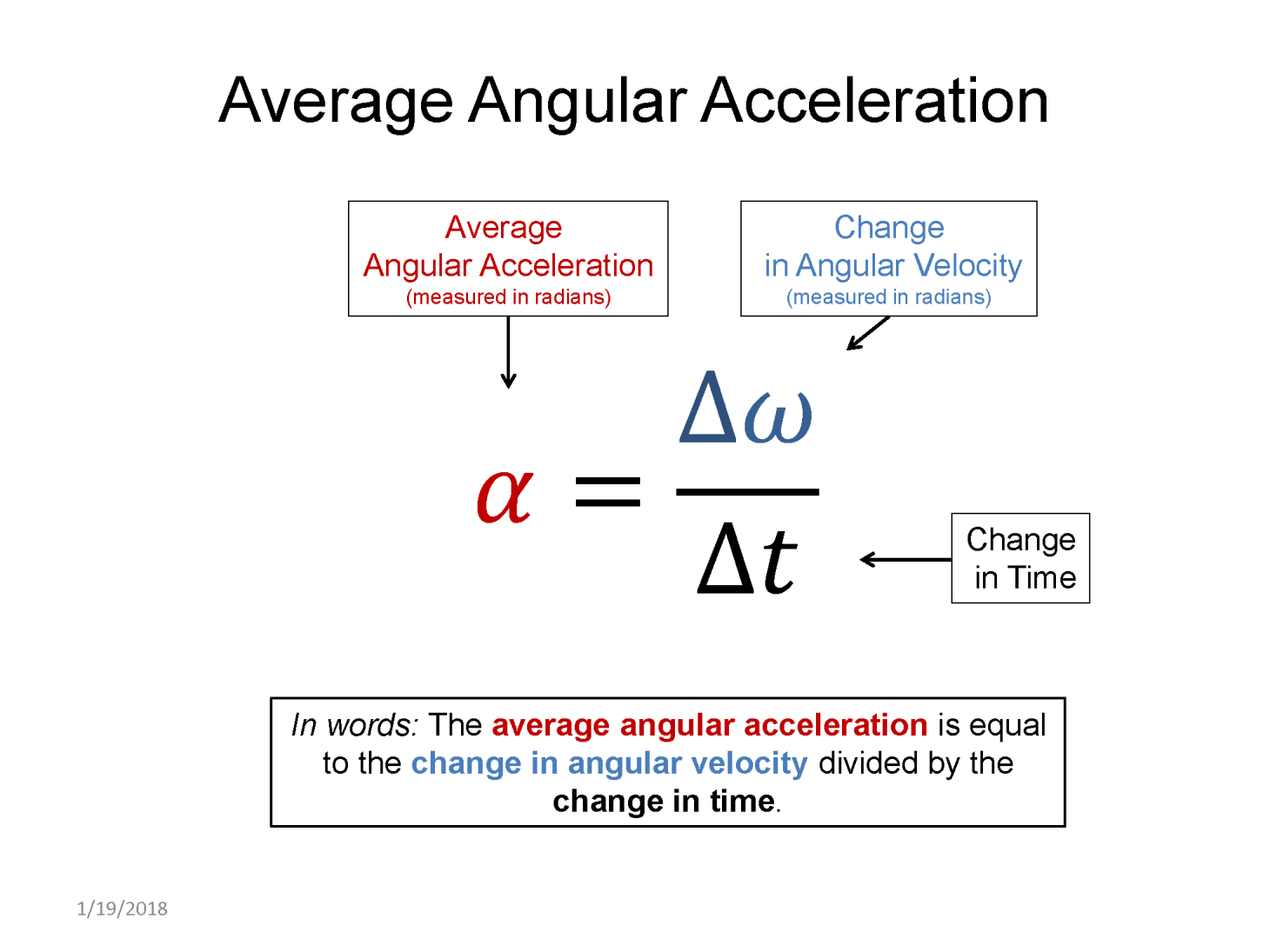
Just as we learned relationships between the linear kinematic variables, so too are there between the rotational kinematic variables. The average angular velocity ($\omega$) is defined as the time rate of change of the angular position.

$\overline{\omega} = \frac{\Delta \theta}{\Delta t}$

Similarly, the average angular acceleration ($\alpha$) is defined as the time rate of change of the angular velocity.

$\overline{\alpha} = \frac{\Delta \omega}{\Delta t}$

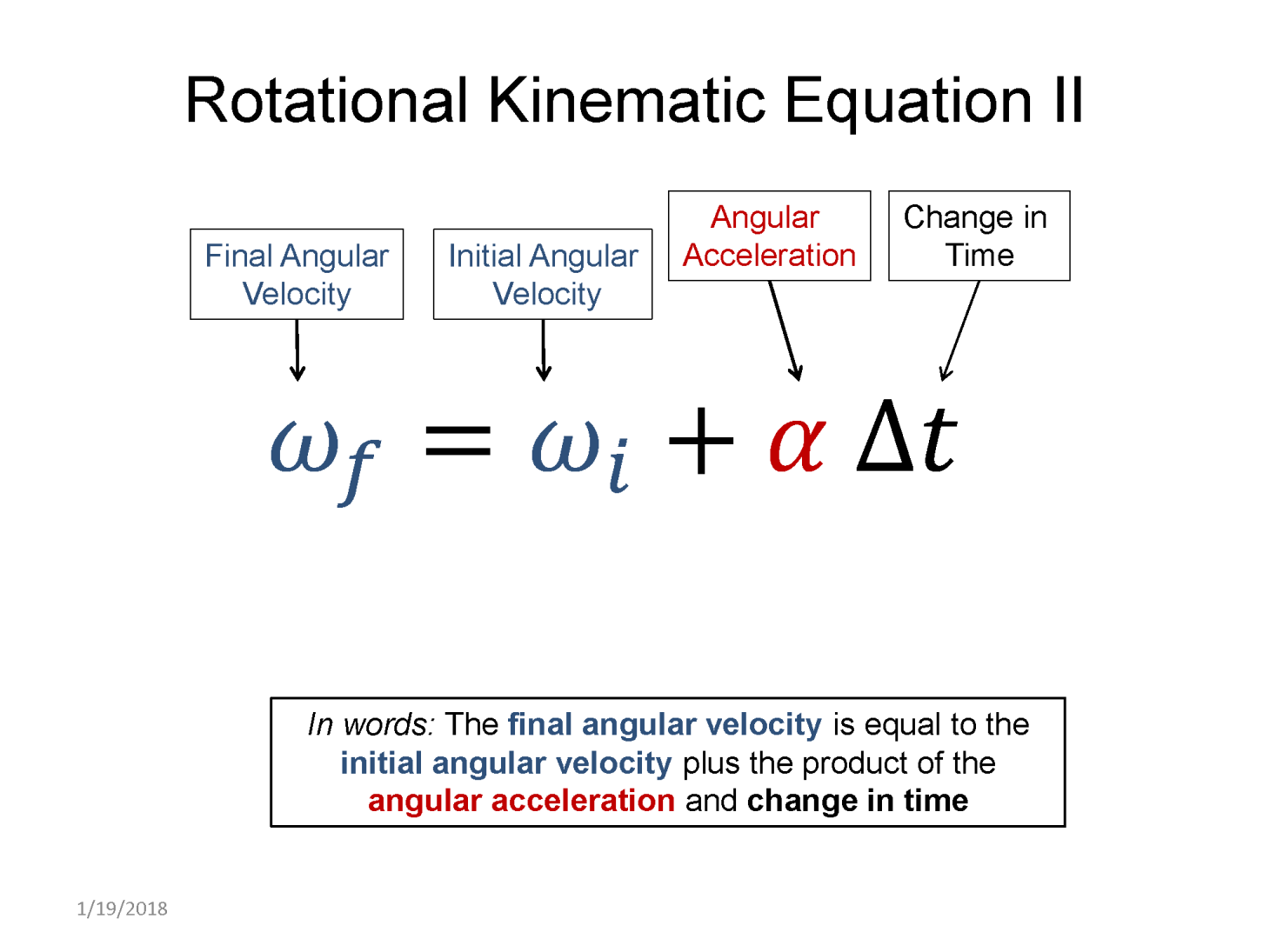
Rotational Kinematic Equations: If all of this looks familiar, it should as it is form like to the linear kinematic variables (x,v,a,t). Form like means that the equations take on the exact same form, replace $\omega$ with $v$ and $\Delta \theta$ with $\Delta x$ and you have the equation for linear velocity in 1D. So it may not be a surprise then if the kinematic equations for constant acceleration also take on the same form for both the angular and linear quantities.

(i) $\Delta \theta = \omega_i \Delta t + \frac{1}{2} \alpha \Delta t^2$

(ii) $\omega_f = \omega_i + \alpha \Delta t$

(iii) $\omega_f^2 = \omega_i^2 + 2 \alpha \Delta \theta$

With all the equations for both the linear and angular variables being form like, this leads the way to using all the techniques learned in solving kinematics problems for linear variables. We decided to omit a discussion about the vector nature of angular quantities and we get away with this by limiting our cases to rotation in a plane. By doing this we can simply use a convention for positive and negative. So, an object traveling in counter-clockwise (CCW) direction will be considered to have a positive angular velocity ($\omega$). That means the object's change in position must also be positive. Conversely if it's traveling in the clockwise (CW) direction, $\omega$ would be a negative quantity. For determining the sign of the angular acceleration, you use the lessons learned from linear acceleration in 1D.

If the object is slowing down, the angular acceleration has the opposite sign of the angular velocity.

If the object is speeding up, the angular acceleration has the same sign as the angular velocity.

An example of where the object's speed is changing, and thus its angular acceleration ($\alpha$) is not zero, would be if an object was slowing down while moving from the initial to final position. A proper physical representation needs to add information about the initial and final angular velocity and the angular acceleration during that time. Time is not always useful in these representations unless there are multiple stages to differentiate between. An updated physical representation is below.

Image

Going Between Angular and Linear: Now that we see what the rotational kinematic variables are, and how the equations for constant acceleration allows you to use them to find instantaneous values, it's important to see how they can also be used to find their linear counterparts. Some problems may state what the initial and final angular velocities are, and the change in angle during that motion, then ask for the time. In that case you would not have to use any of the linear quantities to solve the problem. Although it then asks what the linear speed was at the end of the motion, you'd have to use the following relationships below.

Change in angular position ==> Distance traveled: $s=\Delta \theta r$

Angular velocity ==> speed: $|\overrightarrow{v}| = v_t = \omega r$

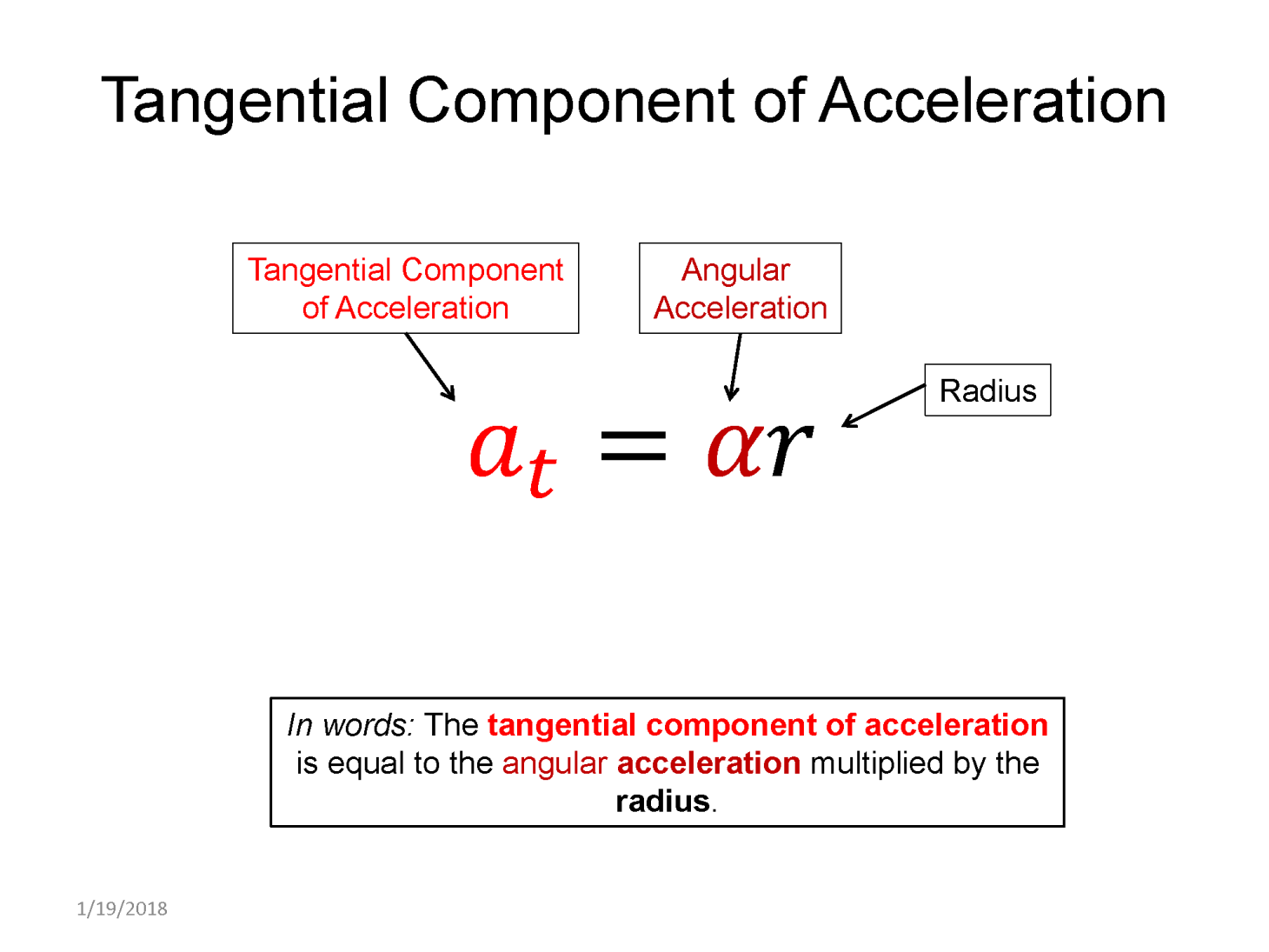
Angular acceleration ==> Tangential component of linear acceleration: $a_t = \alpha r$

The linear coordinate system we use in this case is one with a radial inward direction ($\widehat{r}$), a CCW tangential direction ($\widehat{t}$), and a direction perpendicular to those two ($\widehat{z}$). This means that since the object is always traveling tangent to the circle, the linear velocity has zero radial or z components - the speed of the object is equal to the tangent component of its linear velocity.

$\overrightarrow{v}=\langle v_r, v_t, v_z \rangle = \langle 0, \omega r, 0 \rangle$

For the angular acceleration, using the same $\widehat{r}$,$\widehat{t}$, and $\widehat{z}$, coordinate system, the object has zero z component to its acceleration. If you recall though it does have a radial component equal to the square of its speed divided by the radius of the circle its traversing ($a_r = \frac{v^2}{r}$). The full linear acceleration is thus:

$\overrightarrow{a}=\langle a_r, a_t, a_z \rangle = \langle \frac{v^2}{r}, \alpha r, 0 \rangle$

Key Equations and Infographics

Required Videos

OpenStax Section 10.1 | Angular Acceleration

Image

OpenStax Section 10.2 | Kinematics of Rotational Motion

Image