Lecture 2 | Multi & Single Slit, Spectroscopy | BoxSand

Wave Optics | Multi and Single-Slit Interfernce

Multi-Slit Interference

A preferred experiment to measure the wavelength of light is the multi-slit experiment. Instead of only two openings, you have multiple slits, which has the effect of sharpening the constructive interference peaks. The multi-slit apparatus is called a diffraction grating when light passes through it and a reflection grating when light reflects off of it. Below is a diagram for a diffraction grating.

Physical representation of parallel horizontal rays of light shining through multiple openings and being deflected downward. The distance between the openings is labeled as d. The angle of deflection after the openings is show to be theta. The path length difference is labeled as delta l and is equal to d multiplied by the sine of theta.

Here the first slit interferes with the second and the second with the third, and so on. Each subsequent slit has the same PLD condition as for a double slit. It is a bunch of double slits slightly shifted from each other. The result is a sharper set of interfrence fringes and the same conditions and equations as for the double slit.

Single Slit Interference

Once you have a wave picture of light and understand superposition, the inteference patterns of the double slit and muti-slit setups are not wierd. But what's truely a mind bender is when passing light through a single slit you also observe an interference pattern, although one different from the double slit. To understand this effect you must consider Huygens Principle which states that each point on a wavefront can act as a new spherical source (left figure).

The physical representation illustrates the propagation of a plane wave. It features several vertical and curved lines. Two parallel vertical magenta lines on the left represent the initial wave front. To the right, several concentric magenta semicircles represent the spherical wavelets originating from magenta points on the initial wave front. These points are evenly spaced along the vertical line. The wave front at a later time is shown as a tangential line to all the wavelets.

The physical representation depicts a diagram of six parallel lines, labeled 1 through 6, at regular intervals. These lines are slanted diagonally and oriented in a top-right direction. A vertical line intersects these at designated points. At the top and bottom of the vertical line, there are rectangular blocks. The intersections occur between these blocks, marked by red dots. A dashed line indicates an angle, θ, between the vertical line and the diagonal lines. A red segment connects two of the intersections between lines labeled 2 and 3. The vertical distance between intersections is labeled as "a/2." A blue dashed arc represents the path between lines 2 and 1, labeled as "Δr_{12}."

Each new spherical source interfere to create the next wavefront, which can then be a set of new spherical sources. This may seem counter intuitive and we don't know if light really behaves this way, but if modeling it this way is consistent with observation, we can't throw it out as a possibility. In fact this model then helps us understand the single slit interference pattern. Now waves generated at the top of the source can interfere with waves on the bottom of the source (figure above on the right).

The interference pattern is similar in that there are light and dark regions but it differs in the locations of the maxima and minima.

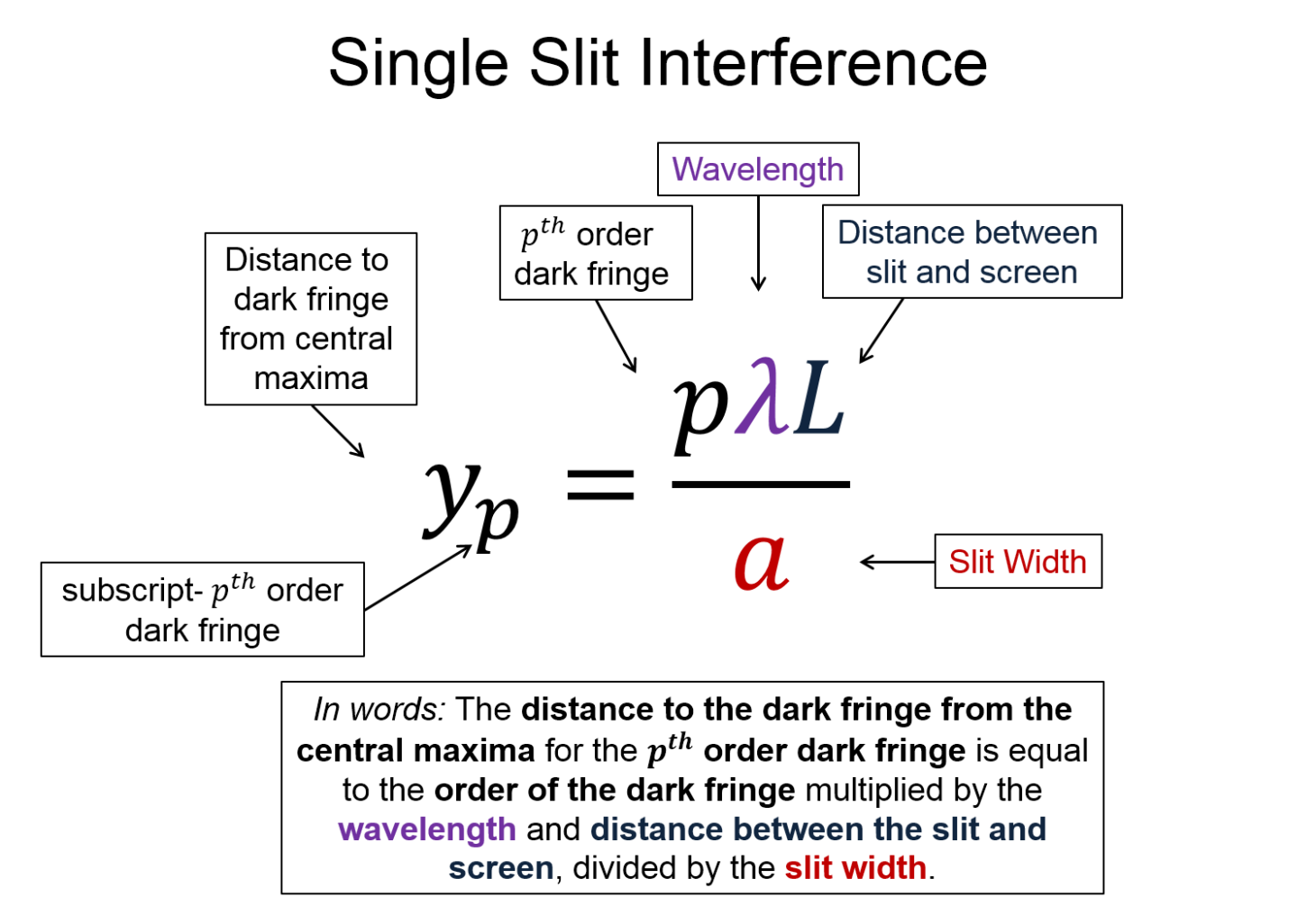
The image depicts a diagram related to the diffraction of light through a single slit. On the left side, there are three mathematical equations. To the right, there is a diagram showing a single slit on the left, labeled "Single slit," and a screen on the right labeled "Screen." A wave pattern on the screen represents light intensity. Dashed lines from the slit to the screen indicate angles and positions of maxima and minima. Labels on the diagram include "Central maximum" and indicate various positions denoted by letters "p=1" and "p=2." The distance "w" representing width, and angles are marked as well. A horizontal axis is labeled "Light intensity."

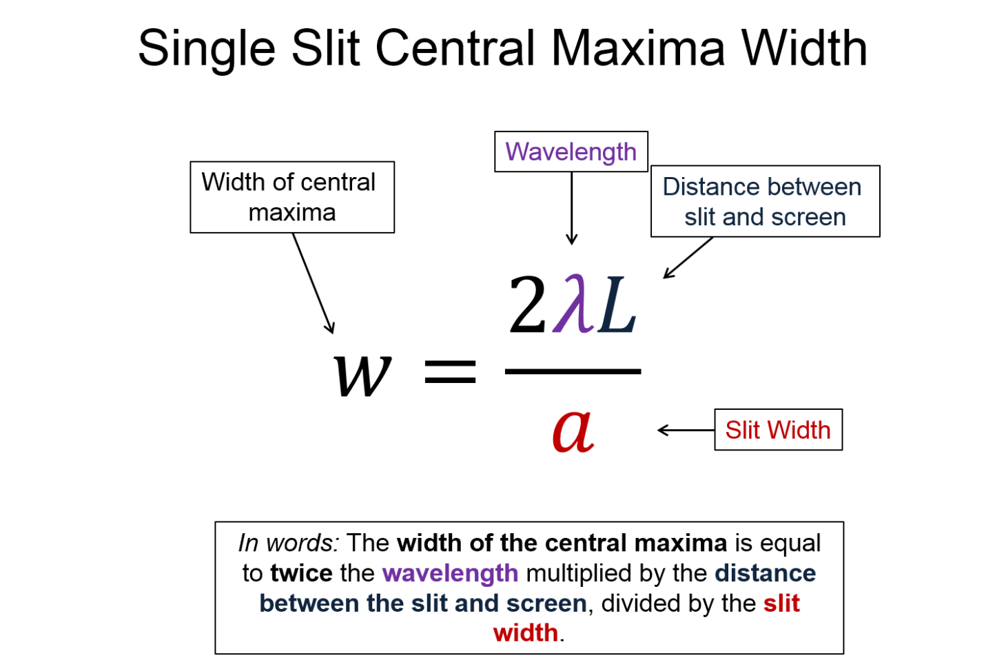
The interference is also often described by the locations of the destructive interference points. Here the integer p is describing the order of the dark fringes. The width of the central maximum (w) can be found by doubling y1.

To see the difference between the single and the double slit interference patterns, along with the effects of sharpening the fringes by adding more slits, refer to the figure below.

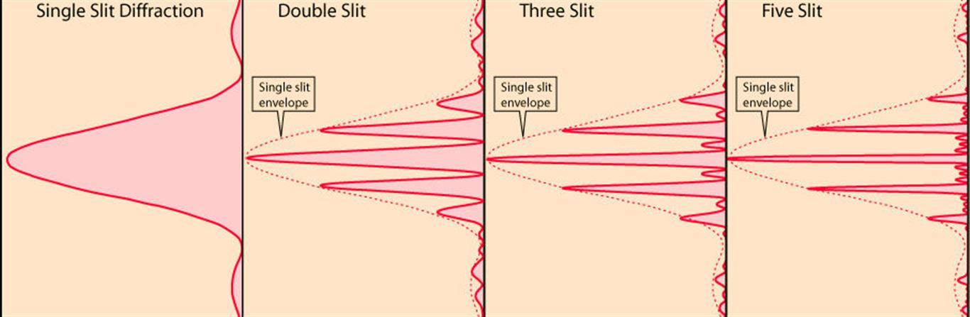
The physical representation is divided into four sections horizontally, each titled "Single Slit Diffraction," "Double Slit," "Three Slit," and "Five Slit." It visually represents diffraction patterns in red lines on a beige background. In the "Single Slit Diffraction" section, a broad central peak is shown. The "Double Slit" section displays multiple narrower peaks within a broad envelope, with text indicating the "Single slit envelope." The "Three Slit" and "Five Slit" sections show increasingly complex patterns with more peaks, also inside a single slit envelope.

Single-Slit Interference Mathematical Model

To explain why the mathematical model for single slit interference uses destructive interference fringes, unlike either of the double or multi-slit models, we need to consider several special cases illustrated below.

We will split the single slit into successively more equal sections. The first of which we will consider is the slit as a whole. We see that light incident on the slit can simply shine directly through the slit onto a screen opposite the slit. Since these rays are all parallel with no path length difference between them, they will interfere constructively and we will find a central bright spot on the screen directly opposite the slit.

Physical representation that depicts a single slit of width a. Parallel horizontal rays shine through the slit to the right.

To find the angle at which the first destructive interference, dark, fringe occurs, we will divide the single slit of width a into equal sections of width a/2. Additionally, we will consider waves which have been diffracted up at a slight angle. We will examine three waves, one from the top edge of the slit (labeled with a number 1), another from the middle of the slit (labeled with a number 2), and a final wave from the bottom edge of the slit (labeled with a number 3). We will choose an angle such that there is a path length difference of one half of a wavelength between the top and middle waves. We can then examine the triangle made near the start of waves 1 and 2. The sine of the shown angle is the opposite side (1/2 lambda) divided by the hypotenuse (a/2). Simplifying this, we find the equation given between the images. The "1" before the lambda is emphasized because this will eventually be our variable labeled "p". This is the p = 1 dark fringe, which is the first fringe on either side of the central bright spot.

The image illustrates three light paths emerging from a vertical black line on the left, which represents a single slit. Three blue lines, labeled 1, 2, and 3, extend diagonally to the right, each forming an angle θ with the horizontal dotted lines. The spacing between the lines is denoted by "a" on the left side, with half the distance ("a/2") labeled between lines 1 and 2. A red line within the slit area indicates the path length difference (PLD), labeled "PLD = 1/2 λ". To the right, there are mathematical expressions: "sin θ = λ/a2 = λ/2" and "1 λ = a sin θ".

Animated image that shows three main rays angled up and to the right shining through a slit of width a. The distance between each ray is shown to be a/2. Each frame of the animation shows an additional set of rays the same distance apart in the same direction being added to the rays shown. In the end there are 7 parallel rays.

To see that this gives a destructive interference fringe, we can look at the animated gif. For every wave between waves 1 and 2, there is a corresponding wave between 2 and 3 which starts a distance a/2 away, and has a path length difference of one half of a wavelength, thus causing destructive interference.

Next we look at what happens when we divide the single slit into three equal sections of width a/3 and perform the same procedure as above. The diffraction angle needs to increase in order to give the same path length difference of lambda / 2. We find that the resulting equation might represent a "p" value of 3/2. This doesn't fit the mathematical model presented above, so this is a hint that this situation doesn't quite work out!

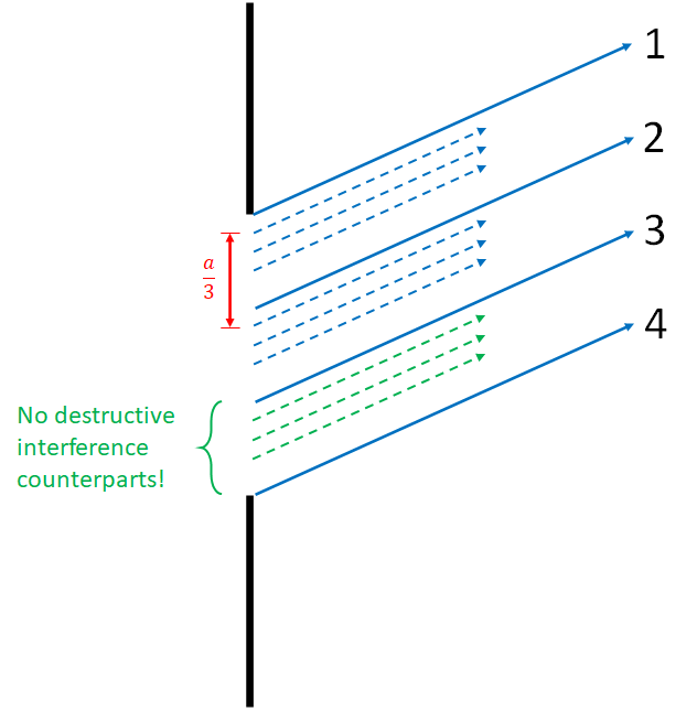
To see that this case is a little funny, look at the image on the right, which shows that as in the first case, for every wave between waves 1 and 2 there is a wave between 2 and 3 which results in destructive interference. However, there is another whole section between waves 3 and 4 which do not have corresponding destructive interference. This means that some light does get through the slit at this angle, and we do not see a destructive interference at this angle. Note that in actuality it is not just the bottom set of waves that get through, there is actually partial destructive interference all around. But that image is a useful conceptual picture to show that there is not complete destructive interference happening as there would be for a dark fringe.

Finally, we look at what happens when we divide the single slit into four equal sections of width a/4. We see that for this case, we arrive at a nicer mathematical model with a "p" value of 2. We also see, in the image on the right, that there are now two sets of two regions which each destructively interfere with each other. This results in the p = 2 dark fringe.

We can repeat this process to find that the p = 3 case will come from dividing the single slit into 6 even sections. From here we can generalize this process to describe the angle of dark fringes from a single slit. We find that the mathematical model is p lambda = a sin(theta), where p = 1, 2, 3, etc. Note that p starts at 1, where m started at 0 for the double and multi-slit mathematical model. The single slit mathematical model also finds the locations of the dark fringes.